
Summary
ConeForest is a random-partition anomaly detector built to run as a few array operations on a GPU. On 48 tabular datasets it is as accurate as Isolation Forest, xStream and Half-Space Trees: no test separates the five. It is much faster than all of them.
| Model | ROC-AUC | AUC-PR | Speed against ConeForest |
|---|---|---|---|
| iForest (sklearn) | 0.767 | 0.401 | 157× slower |
| iForestGPU (cuML) | 0.765 | 0.411 | 12.5× slower |
| ConeForest | 0.764 | 0.398 | 0.7 ms on small sets |
| xStreamGPU (our JAX port) | 0.762 | 0.397 | 17× slower |
| HSTreesGPU (our JAX port) | 0.761 | 0.397 | 2.8× slower |
What the study found beyond the headline:
- It is not more accurate. The claim is “same accuracy, far less time”.
- The score matters more than the partition. In a step-by-step ablation from xStream to ConeForest, only one step is significant: replacing xStream’s score with ConeForest’s (+0.018 ROC-AUC). The speed comes from a different step, which gives most of that gain back.
- The score splits into a density part and a geometry part. The geometry part is a built-in “distance from the centre of the range” penalty. Synthetic checks confirm it to a rank correlation of 0.992.
- Where the cuts are drawn decides what kind of anomaly is found. Cuts uniform in the range find far-out magnitudes. Cuts at sample quantiles ignore the marginals and find broken dependence. Each fails at the other’s task.
- One approximation in our theory sketch failed its check, and we say where.
The implementation is available as a Python package: coneforest 0.1.0 on PyPI; the source is at git.sr.ht/~divanov/coneforest.
The design
ConeForest is an ensemble of b = 256 random oblivious trees. Oblivious means every node at a given level uses the same feature and the same threshold. A tree of depth K is then just K (feature, threshold) pairs, and a row’s leaf is a K-bit code.
Fit, per tree:
- Draw
psitraining rows (tuned over {128, 256, 512}; all rows if there are fewer). - Set the depth to
K = ceil(log2(m)), withmthe sample size. That is 7 to 9. - For each of the K levels, draw a feature with replacement, and a threshold uniform in that feature’s [min, max] over the tree’s sample. Cuts are in raw feature space, with no scaling or rank transform.
- Give every sample row its K-bit code: bit j is 1 when the row is above threshold j. Count rows per code. The low j bits of a code are the row’s cell at depth j, so summing the count table over the high bits gives the counts at every depth.
- For each cell at each depth, take the smoothed log mass
log((count + 1) / (m + 2)). - For each of the 2^K full codes, store one number: minus the mean of the log masses of its K prefix cells.
Score a row: compute its K-bit code in each tree, look up the stored number, and average over trees.
score(x) = mean over trees and depths l = 1..K of −log((countl(x) + 1) / (m + 2))
count_l(x) is the number of the tree’s sample rows in x’s cell after l cuts. High score means few rows share x’s cells, at every scale.
The core is short. This is the build, in JAX, lightly trimmed:
feats = random.randint(k_feat, (b, K), 0, d)
S = X[sub[:, :, None], feats[:, None, :]]                      # (b, m, K)
lo, hi = S.min(axis=1), S.max(axis=1)
thr = lo + random.uniform(k_thr, (b, K)) * (hi - lo)

weights = (1 << jnp.arange(K)).astype(jnp.int32)
codes = jnp.sum((S > thr[:, None, :]) * weights, axis=2)       # (b, m)
table = jnp.zeros((b, 1 << K), jnp.int32).at[jnp.arange(b)[:, None], codes].add(1)
flat = jnp.concatenate(
    [table.reshape(b, 1 << (K - j), 1 << j).sum(axis=1) for j in range(1, K + 1)], axis=1
)
log_mass = jnp.log((flat + 1.0) / (m + 2.0))
and this is all of scoring:
codes = jnp.sum((X[:, feats] > thr[None]) * weights, axis=2)   # (n, b)
return jnp.mean(cell_score[jnp.arange(b)[None, :], codes], axis=1)
Why it is fast.
- Fitting touches
b × psirows, whatever the size of the training set. - Scoring a row costs
b × Kcomparisons andbtable lookups. There is no tree traversal and no branching, so it batches as one gather. - The model is small:
b × Kfeatures and thresholds, and ab × 2^Kscore table (at most 256 × 512 numbers).
How it differs from its relatives.
| Tree shape | Cut | Rows counted | Score | |
|---|---|---|---|---|
| iForest | per-node feature and cut | uniform in the node’s range | subsample | path length to isolation |
| HS-Trees | per-node feature | midpoint of the node’s workspace | reference rows | mass × 2^depth at the terminal node |
| xStream | oblivious, on random projections | equal-width grid, halved on each reuse of a feature | all training rows | min over depths of log2(1 + count) + depth |
| ConeForest | oblivious, raw features | one uniform cut per level in the sample’s range | subsample of psi | mean over depths of −log mass |
xStream’s half-space chains are the closest prior work: they are also oblivious and also draw features with replacement. ConeForest’s differences are the binary random-threshold cut, the per-tree subsample, the mean-of-log-mass score, and the lookup table.
How we evaluated
- Data. 48 datasets: the 47 “classical” tabular datasets of ADBench, plus arrhythmia.
- Splits. 10 runs per dataset. Each run splits 60 / 20 / 20 into train, validation and holdout within each class, so every part has anomalies. Models fit on the training part without labels; it contains anomalies.
- Tuning. 10 Optuna trials per model per run, choosing the setting with the best ROC-AUC on the validation part. The search spaces are small: ConeForest
psiin {128, 256, 512}; iForest 100 to 200 trees and 256 or “auto” samples; xStream depth in {10, 15, 25}; HS-Trees ψ in {125, 250, 500}. COPOD has nothing to tune. - Metrics. ROC-AUC and AUC-PR (average precision) on the holdout part, averaged over runs, then over datasets.
- Statistics. Models are ranked per dataset on their mean score. We report the Friedman test, the Nemenyi critical difference, and pairwise Wilcoxon signed-rank tests over datasets with Holm correction.
- Timing. Fit plus scoring of the holdout part with the tuned setting, median of 10 runs. JAX compile time is not included. All models run on the GPU, except sklearn’s iForest.
Baselines. sklearn’s IsolationForest is the reference. cuML’s GPU IsolationForest is the fair speed comparison. COPOD, xStream and HS-Trees are our own JAX ports, so that every method gets the same GPU treatment:
- COPOD follows pyod’s implementation; scores match pyod’s to 3e-7.
- xStream follows the authors’
python/Chains.py: exact counts, 100 chains, projection to 100 features. It runs in static mode and counts every training row. - HS-Trees follows the IJCAI 2011 paper’s terminal-node score, with 100 trees, each of depth 15. The reference counts come from ψ training rows, not a stream window.
Both tree ports were checked in float64 against the reference code (all 16 checks pass). On the http dataset, the float32 GPU path gave 0 count mismatches in 900,000 cells.
Results
Accuracy
| Model | ROC-AUC | AUC-PR |
|---|---|---|
| iForest | 0.767 | 0.401 |
| iForestGPU | 0.765 | 0.411 |
| ConeForest | 0.764 | 0.398 |
| xStreamGPU | 0.762 | 0.397 |
| HSTreesGPU | 0.761 | 0.397 |
| COPODGPU | 0.746 | 0.357 |
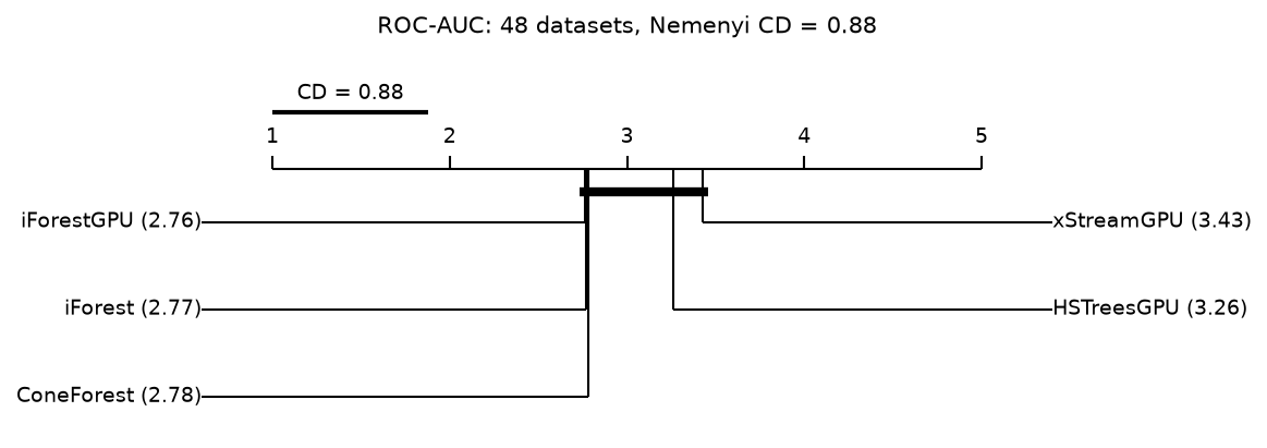
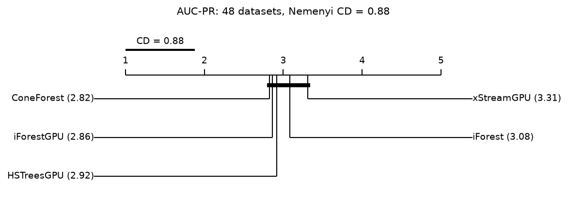
There is no detectable difference among the five tree methods.
| ConeForest | iForest | iForestGPU | xStreamGPU | HSTreesGPU | Friedman p | |
|---|---|---|---|---|---|---|
| Mean rank, ROC-AUC | 2.78 | 2.77 | 2.76 | 3.43 | 3.26 | 0.095 |
| Mean rank, AUC-PR | 2.82 | 3.08 | 2.87 | 3.31 | 2.92 | 0.54 |
The Nemenyi critical difference is 0.88, larger than any gap in mean rank. No pairwise Wilcoxon-Holm test is significant.
Speed
- Against iForest. ConeForest is faster on all 48 datasets: 157× faster than sklearn’s iForest (21 to 350×), and 12.5× faster than cuML’s (2.9 to 19×).
- Absolute times. About 0.7 ms on small datasets, 2.3 ms on those over 100,000 rows, and 35 ms on census (500 columns).
- Against the GPU ports. Taking the per-dataset ratio of median times and the geometric mean over datasets, xStreamGPU is 17× slower (4.3 to 6400×) and HSTreesGPU 2.8× slower (0.95 to 4.6×; slower on 47 of 48). xStream counts every training row, so it takes 0.6 to 14.6 s on the seven datasets over 200,000 rows.
Where ConeForest loses
- http, AUC-PR. 0.425 against 0.95 to 0.995 for the others, at the same ROC-AUC of 0.995. The anomalies are 22 distinct rows with
src_bytesat the top of its range. ConeForest’s top ranks fill with normal rows from the tail ofdst_bytesinstead. Ties do not explain it, and neither does contamination of the training data. An open hypothesis: one global threshold per level is coarser than iForest’s cuts, which adapt to each node’s range. - Wilt. 0.362 ROC-AUC against 0.467.
- optdigits and landsat. 0.05 to 0.07 below.
Ablation: which part of ConeForest matters?
We walked from xStream to ConeForest one change at a time, on the same 48 datasets and protocol. Steps A1 to A3 keep xStream’s 100 chains, count every training row, and tune depth over {10, 15, 25}. The p-values are two-sided Wilcoxon tests of ROC-AUC against the previous step.
| Step | ROC-AUC | AUC-PR | Median time | Against the previous step |
|---|---|---|---|---|
| A0 xStreamGPU | 0.762 | 0.397 | 4.7 ms | |
| A1 no projection (raw features) | 0.763 | 0.397 | 3.8 ms | 31/48 wins, p = 0.13 |
| A2 + ConeForest’s score | 0.781 | 0.404 | 3.8 ms | 30/48, p = 0.007 (Holm 0.037) |
| A3 + one uniform binary cut per level | 0.774 | 0.409 | 3.3 ms | 19/48, p = 0.12 |
| A4 + psi rows per tree, depth ceil(log2 psi), 100 trees | 0.762 | 0.396 | 0.6 ms | 18/48, p = 0.047 (Holm 0.19) |
| A5 ConeForest, 256 trees | 0.764 | 0.397 | 0.6 ms | 26/48, p = 0.14 |
| ConeForest with mirrored cuts | 0.770 | 0.399 | 0.55 ms | against ConeForest: 21/48, p = 0.35 |
- The score is the one significant step. Swapping xStream’s min-over-depths for the mean of −log mass adds 0.018 ROC-AUC and survives Holm correction. landsat, skin and fault gain about 0.11 each. No step changes AUC-PR significantly.
- The subsample gives the speed and costs accuracy. A4 takes the median from 3.3 ms to 0.6 ms (A2 needs 14 s on donors) and loses 0.012 ROC-AUC.
- A4 is not one change. Besides the subsample it changes the depth, the range the cuts are drawn from, and the scoring path (table lookup instead of a search over all rows). These effects are not yet separated.
- A2 is not a clear winner over ConeForest. It beats ConeForest on only 23 of 48 datasets (p = 0.24). A few large gains drive its mean.
- Removing xStream’s projection makes no significant difference (p = 0.13).
The open engineering question follows directly: a variant that keeps A2’s score gain at A4’s speed.
Uniform, quantile and mirrored cuts
We tried two other ways to place thresholds, on the same splits.
- Quantile cuts. The threshold is the midpoint of two neighbouring sorted sample values, at a uniformly random rank.
- Mirrored cuts. Half the trees use uniform cuts and half use quantile cuts. Each pair shares its sample, features and random draws.
| Cuts | ROC-AUC | AUC-PR |
|---|---|---|
| Uniform (ConeForest) | 0.764 | 0.398 |
| Quantile | 0.763 | 0.361 |
| Mirrored | 0.770 | 0.399 |
None of these differences is significant (quantile against uniform: p = 0.52 on ROC-AUC, p = 0.11 on AUC-PR; mirrored against uniform: p = 0.35). The means hide large moves on single datasets:
- Quantile cuts help Wilt (0.36 → 0.57 ROC-AUC), donors, PageBlocks, backdoor, skin and vowels.
- They hurt http (AUC-PR 0.425 → 0.131), WDBC, musk, shuttle, thyroid and Stamps.
- Mirrored cuts land between the two on 36 of 48 datasets, at the same run time.
The two schemes look complementary. The theory sketch below says why.
Theory sketch: the score through Sklar’s theorem
This is a sketch, not a proof. Each step is marked exact or heuristic, and the checks in the next section test it.
Setup. X in ℝd has density f, marginal CDFs Fj with densities fj, and copula density c. Sklar’s theorem: f(x) = c(F1(x1), …, Fd(xd)) · Πj fj(xj). A tree draws features j1…jK with replacement and thresholds t1…tK. Al(x) is the cell of x after l cuts, an axis-aligned box. The population score is
S(x) = Etree[(1/K) Σl −log P(Al(x))]
The code’s (count + 1) / (m + 2) is the posterior mean of P(Al) under a uniform prior.
1. Mass = average density × volume (exact). For any box A, P(A) = f̄A · vol(A), with f̄A the mean of f over A. So −log P(Al(x)) = −log f̄Al(x) − log vol(Al(x)). The volume is a product of interval lengths, so its log is a sum over features:
S(x) = [−log of the cell-averaged f, over scales] + Σj h(position of xj)
- h(t) = E[−log length of the interval around t]. It depends only on how cuts are drawn, not on the data.
- With one uniform cut on [0, 1], h(t) = 1 − H(t), with H the binary entropy in nats. It is U-shaped: 0.31 at the centre, 1 at the edges.
- With many cuts per feature, h flattens to a constant in the interior. ConeForest has about 8 cuts spread over d features, so it sits in the few-cuts regime and the U-shape matters.
So the score has a data-free geometry term: a bounded penalty for sitting near the edge of the range.
2. Quantile cuts see only the copula (exact at population level). Take thresholds at Fj−1(v), with v uniform. In rank coordinates u = F(x) the cuts are uniform on [0, 1]d, and a cell’s mass is the copula’s mass of a box:
SQ(x) = [−log of the cell-averaged c at u, over scales] + Σj h(uj)
The score depends on the copula and the ranks only. The marginals drop out. The geometry term stays, as a bounded, distribution-free penalty on extreme ranks.
3. Uniform cuts see the full density (heuristic: small cells). Rescale each feature to z in [0, 1] by its range. The same identity holds with f in place of c:
SU(x) ≈ −log c(u) − Σj log fj(xj) + Σj h(zj)
4. Mixing gives tempered marginals (heuristic). With a fraction λ of uniform-cut trees and 1 − λ of quantile-cut trees:
Sλ(x) ≈ −log c(u) − λ Σj log fj(xj) + geometry
This is −log of c · Πj fjλ: the joint density with its marginals tempered. λ = 1 is ConeForest, λ = 0 is quantile cuts, λ = ½ is mirrored cuts. Mixing tree types only reaches λ in [0, 1].
5. Why the mean of logs should beat xStream’s min (a claim to prove).
- Telescoping: −log P(Al) = Σi≤l −log P(Ai | Ai−1). The mean over depths is then Σi wi · (surprisal of cut i), with wi = (K − i + 1) / K. The score is a weighted code length for locating x, with early cuts weighted most.
- xStream’s score is the min over depths of log2(1 + count) + depth. Once a cell is empty, this is roughly the depth at which x is isolated. It uses one extreme value, so it takes few distinct values and ties often.
- The claim: the mean uses all K levels with bounded terms, so it has lower variance and finer resolution than the min. This is the ablation’s A1 → A2 step, and it is not yet proven.
Caveats.
- With d much larger than K, a tree cuts at most K features. The rest integrate out, so each tree scores a random low-dimensional marginal. Only dependence among up to K features is ever seen.
- This is not a consistent density estimator: K = log2 m leaves about one row per deepest cell. The honest theorem is concentration of the score around S(x) as trees grow, not convergence to −log f.
- Empirical quantile cuts are midpoints of sample values, so invariance to monotone maps may be only approximate in finite samples.
Testing the sketch on synthetic data
Each check uses 256 trees of 256 rows and 20,000 training rows. Correlations are Spearman on 4,000 test rows. AUC-PR checks score 20,000 test rows and average 3 seeds.
The geometry term is real. With independent features and five different marginals (normal, lognormal, uniform, exponential, t3):
| Comparison | Spearman |
|---|---|
| Quantile score against the predicted geometry term | 0.992 |
| Quantile score against Σj (1 − H(uj)) | 0.992 |
| Two quantile forests with different seeds | 0.986 |
| Quantile score against COPOD | 0.81 |
| Quantile score against −log f | 0.58 |
| Uniform score against its own Monte Carlo prediction | 0.995 |
The seed-to-seed agreement puts the ceiling for a noise-free target near √0.986 = 0.993, so 0.992 is as good as it can be.
Quantile cuts ignore the marginals. Take the same ranks under normal and under lognormal marginals (Gaussian copula, d = 4, correlation 0.7). Quantile scores correlate at 1.0000 between the two. Uniform scores correlate at 0.59.
Uniform cuts find far-out magnitudes; quantile cuts cannot. 1% of rows are shifted by k standard deviations in one of five normal features, in training and test data:
| Shift k | Uniform, AUC-PR | Quantile, AUC-PR |
|---|---|---|
| 3 | 0.118 | 0.037 |
| 5 | 0.452 | 0.043 |
| 10 | 0.920 | 0.044 |
| 100 | 1.000 | 0.044 |
The geometry term is bounded, so with quantile cuts a far outlier scores no higher than the merely most extreme row.
Quantile cuts find broken dependence; uniform cuts cannot. 1% of rows get each feature from a different row. That keeps the marginals and breaks the dependence:
| Pairwise correlation | Uniform, AUC-PR | Quantile, AUC-PR |
|---|---|---|
| 0.7 | 0.018 | 0.243 |
| 0.95 | 0.028 | 0.705 |
With lognormal marginals the quantile numbers are identical; uniform gets 0.015 and 0.020.
Monotone transforms. After a log transform of lognormal data (Gaussian copula, d = 4, correlation 0.5), quantile scores keep their ranking (Spearman 1.0000 to four decimals) but move by up to 0.023. The cause is not traced: midpoint cuts and float32 rounding are both candidates. Uniform scores change a lot (Spearman 0.56).
The small-cell approximation fails. We tested it on the quantile score, replacing step 2’s cell-averaged copula density by the pointwise −log c:
- On the Gaussian copula, −log c + geometry correlates with the quantile score at only 0.24. Geometry alone gets 0.73.
- A least-squares fit on both terms explains 76% of the variance, against 46% for geometry alone and a seed ceiling of 96%.
- The fitted weights are 0.096 on −log c and 0.71 on geometry: a ratio of 0.13, where the approximation predicts 1.
- Uniform scores correlate with −log c at −0.33 (normal marginals) and −0.19 (lognormal), where step 3 predicts a positive value.
With about two cuts per feature the cells are large, so the scores see a heavily smoothed density. Steps 3 and 4 rest on this approximation. They need the cell-averaged density of step 1, not the pointwise one.
An unexplained observation. With normal marginals, quantile scores track −log f at 0.96, above uniform cuts (0.83). A hypothesis, not measured: the geometry term acts like a fixed bell-shaped marginal, so quantile cuts behave like density scoring after each feature is mapped to a reference shape.
What these checks suggest about the real data. The synthetic pattern matches the benchmark: quantile cuts gain on Wilt and collapse on http. We have not checked whether Wilt’s anomalies are dependence anomalies or http’s are magnitude anomalies.
Limitations
- No accuracy gain. The result is parity at lower cost.
- Tuning uses labels. The setting is chosen on a labelled validation part. Fully unsupervised use would fix
psi. - Tuning is not seeded. The Optuna sampler had no fixed seed. A rerun with the same splits changed ConeForest’s per-run ROC-AUC on 12 of 48 datasets (by up to 0.029; dataset means by at most 0.003).
- Timing. Compile time is excluded and we report medians. Mean times are inflated, because the last scoring chunk can trigger a recompile inside the timed window.
- Our ports. xStream and HS-Trees are our JAX ports in a static setting, not the authors’ streaming code. The scoring kernels are checked against reference code; the fitting code is not covered by those checks.
- The ablation’s A4 step is confounded, as noted above.
- The theory is a sketch. Steps 1 and 2 are exact at population level. Steps 3 and 4 failed their direct check in the form stated. Step 5 is an unproven claim.
What comes next
- Prove or refute step 5: lower variance of the mean of logs against the min, at a bias we can state, including the role of the +1 / +2 smoothing in empty cells.
- Redo steps 3 and 4 with the cell-averaged density.
- Split A4 into its parts, and look for a variant that keeps A2’s gain at A4’s speed.
- Check the anomaly types in http and Wilt directly, and run ADBench’s synthetic anomaly types: dependency anomalies should favour quantile cuts, global ones uniform cuts.
- Weight depths instead of taking a plain mean, and tune the number of trees.
- Seed the tuner, so that reruns reproduce.
References
- Fei Tony Liu, Kai Ming Ting, Zhi-Hua Zhou. Isolation Forest. IEEE International Conference on Data Mining (ICDM), 2008, pp. 413–422. doi:10.1109/ICDM.2008.17
- Swee Chuan Tan, Kai Ming Ting, Fei Tony Liu. Fast Anomaly Detection for Streaming Data. International Joint Conference on Artificial Intelligence (IJCAI), 2011, pp. 1511–1515. ijcai.org/proceedings/2011/254
- Emaad Manzoor, Hemank Lamba, Leman Akoglu. xStream: Outlier Detection in Feature-Evolving Data Streams. ACM SIGKDD Conference on Knowledge Discovery and Data Mining (KDD), 2018, pp. 1963–1972. cmuxstream.github.io
- Zheng Li, Yue Zhao, Nicola Botta, Cezar Ionescu, Xiyang Hu. COPOD: Copula-Based Outlier Detection. IEEE International Conference on Data Mining (ICDM), 2020, pp. 1118–1123. arXiv:2009.09463
- Songqiao Han, Xiyang Hu, Hailiang Huang, Minqi Jiang, Yue Zhao. ADBench: Anomaly Detection Benchmark. NeurIPS 2022, Datasets and Benchmarks track. arXiv:2206.09426